The Precision Problem
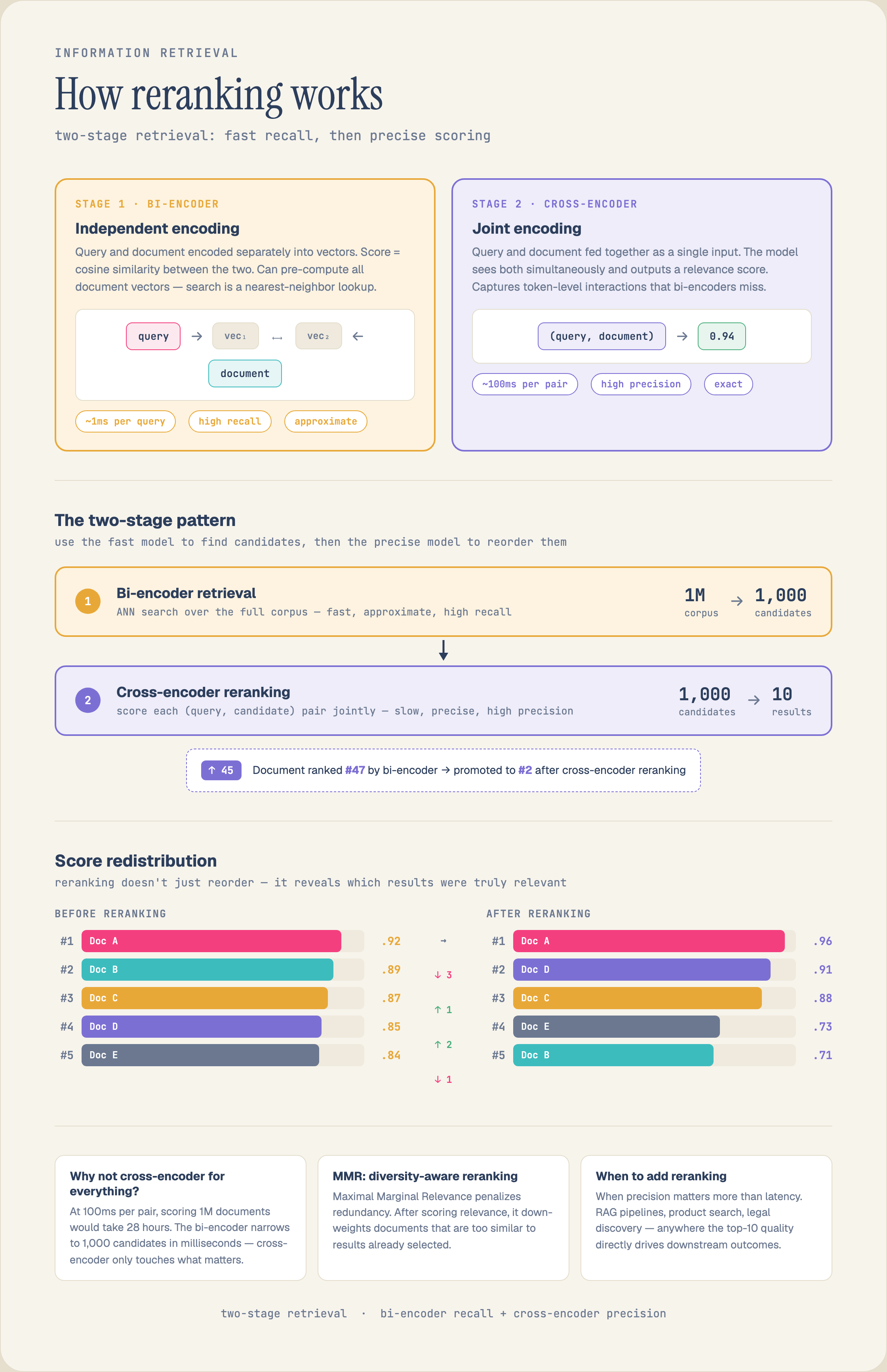
Embedding-based retrieval is fast but imprecise. A bi-encoder embeds the query and each document independently, then compares them via cosine similarity. This works because the embeddings capture semantic meaning -- "quarterly revenue" and "Q3 earnings" end up close together in vector space even though they share no words.
But independent encoding has a fundamental limitation: the query embedding and the document embedding never see each other during computation. The bi-encoder must compress all possible query-relevant information about a document into a single fixed-dimensional vector before it knows what the query will be. This means it can't attend to which parts of a document are relevant to a specific query.
Consider a 10-page financial report. The bi-encoder produces one embedding for the whole document (or one per page/chunk). When you search for "EMEA region growth rate," the embedding must have captured EMEA-related information alongside everything else in the document. If the EMEA discussion is 2 sentences in a 500-word chunk, those 2 sentences contribute a small fraction of the overall embedding -- diluted by the surrounding content about other regions.
A cross-encoder solves this by processing the query and document together. It concatenates them into a single input sequence and runs full bidirectional attention across both. Every token in the query can attend to every token in the document and vice versa. The model can learn that "EMEA region growth rate" in the query should attend specifically to the sentence mentioning "European and Middle Eastern markets grew 12% year-over-year" in the document.
This is why cross-encoder rerankers consistently improve retrieval quality by 5-15% on standard benchmarks. The quality improvement comes from the architectural difference, not from having more parameters or better training data.
Bi-Encoder vs Cross-Encoder: The Architecture
Understanding the difference between bi-encoders and cross-encoders is essential for designing retrieval systems.
Bi-Encoder (Embedding Model)
A bi-encoder processes query and document independently through the same (or separate) encoder networks:
Query: "EMEA growth rate"     Document: "Markets in Europe grew 12%..."
       |                                 |
   [Encoder]                         [Encoder]
       |                                 |
   q_vec (768-dim)                  d_vec (768-dim)
       |                                 |
       +---------- cosine(q, d) ---------+
                       |
                    score: 0.73
The key property: the document embedding is computed once at index time and stored. At query time, only the query needs to be encoded. Then a fast nearest-neighbor search (HNSW, IVF) finds the top-K closest document vectors.
Latency: O(1) per query encoding + O(log N) for ANN search over N documents.
A cross-encoder processes query and document jointly as a single concatenated input:
Latency: O(1) per query encoding + O(log N) for ANN search over N documents.
Cross-Encoder (Reranker)
A cross-encoder processes query and document jointly as a single concatenated input:
Input: "[CLS] EMEA growth rate [SEP] Markets in Europe grew 12%... [SEP]"
       |
   [Transformer with full cross-attention]
       |
   relevance score: 0.91
Every token attends to every other token across both query and document. The [CLS] token's final hidden state (or the logits of a classification head) is the relevance score.
Latency: O(L^2) where L = len(query) + len(document). Must be computed for every query-document pair at query time -- there's nothing to precompute.
This is why cross-encoders can't be the first retrieval stage. Scoring 1 million documents with a cross-encoder at ~5ms each would take 83 minutes per query. But scoring the top 100 candidates from a fast first stage takes only 500ms -- well within interactive latency budgets.
The quality gap between bi-encoders and cross-encoders comes from a specific mechanism: cross-attention between query tokens and document tokens.
In a bi-encoder, the query tokens and document tokens never interact. The query embedding must capture the intent ("find information about EMEA growth") independently. The document embedding must capture all information in the document independently. The only interaction is a single dot product at the end.
In a cross-encoder, query tokens can attend to document tokens at every layer. This enables:
Term weighting. The model learns which document terms are relevant to the specific query. "Grew 12%" is highly relevant when the query mentions "growth rate" but less relevant when the query asks about "executive changes." A bi-encoder can't do this because it doesn't know the query when encoding the document.
Negation handling. "Not applicable to European markets" is semantically close to "applicable to European markets" in embedding space (they share most words). A cross-encoder sees the full context and correctly scores the negated version as irrelevant to an EMEA-focused query.
Multi-hop reasoning. If the query is "which region had the highest growth" and the document discusses several regions, the cross-encoder can compare the growth figures across regions to determine relevance. A bi-encoder encodes each region's data into the same vector and can't do this comparison.
Bi-encoder cosine similarity and cross-encoder scores live on different scales and have different properties.
Cosine similarity (bi-encoder) ranges from -1 to 1. In practice, most retrieval results cluster between 0.5 and 0.9. The scores are relative -- a 0.85 from one query is not comparable to a 0.85 from a different query because the query embedding changes.
Cross-encoder scores are typically log-probabilities or logits from a classification head. Common implementations output the probability that a document is "relevant" vs "irrelevant" by comparing the logits of true/false tokens:
Latency: O(L^2) where L = len(query) + len(document). Must be computed for every query-document pair at query time -- there's nothing to precompute.
This is why cross-encoders can't be the first retrieval stage. Scoring 1 million documents with a cross-encoder at ~5ms each would take 83 minutes per query. But scoring the top 100 candidates from a fast first stage takes only 500ms -- well within interactive latency budgets.
Why Cross-Attention Matters
The quality gap between bi-encoders and cross-encoders comes from a specific mechanism: cross-attention between query tokens and document tokens.
In a bi-encoder, the query tokens and document tokens never interact. The query embedding must capture the intent ("find information about EMEA growth") independently. The document embedding must capture all information in the document independently. The only interaction is a single dot product at the end.
In a cross-encoder, query tokens can attend to document tokens at every layer. This enables:
Term weighting. The model learns which document terms are relevant to the specific query. "Grew 12%" is highly relevant when the query mentions "growth rate" but less relevant when the query asks about "executive changes." A bi-encoder can't do this because it doesn't know the query when encoding the document.
Negation handling. "Not applicable to European markets" is semantically close to "applicable to European markets" in embedding space (they share most words). A cross-encoder sees the full context and correctly scores the negated version as irrelevant to an EMEA-focused query.
Multi-hop reasoning. If the query is "which region had the highest growth" and the document discusses several regions, the cross-encoder can compare the growth figures across regions to determine relevance. A bi-encoder encodes each region's data into the same vector and can't do this comparison.
Score Calibration
Bi-encoder cosine similarity and cross-encoder scores live on different scales and have different properties.
Cosine similarity (bi-encoder) ranges from -1 to 1. In practice, most retrieval results cluster between 0.5 and 0.9. The scores are relative -- a 0.85 from one query is not comparable to a 0.85 from a different query because the query embedding changes.
Cross-encoder scores are typically log-probabilities or logits from a classification head. Common implementations output the probability that a document is "relevant" vs "irrelevant" by comparing the logits of true/false tokens:
score = softmax([logit_true, logit_false])[0]
This produces calibrated probabilities between 0 and 1, where 0.8 genuinely means "80% confident this document is relevant." The calibration property is useful for setting relevance thresholds -- you can filter results below 0.5 confidence rather than guessing a cosine similarity threshold.
However, in production, scores from different reranker models are NOT comparable. A 0.7 from one reranker means something different than a 0.7 from another. If you swap rerankers, you need to recalibrate your thresholds.
Cross-encoder reranking extends naturally to multimodal content. A visual reranker processes the query text concatenated with an image (or document page) through a vision-language model. The cross-attention mechanism works across modalities: text query tokens attend to visual patch tokens.
This is particularly powerful for document retrieval. A scanned PDF page contains text, tables, charts, and layout information. A text-only bi-encoder can only match against extracted OCR text and misses the visual elements entirely. A multimodal reranker sees the page as an image and can match query terms to visual elements:
"revenue breakdown by region" matches a stacked bar chart labeled by region
"signature on page 3" matches a visual signature element
"table with quarterly figures" matches a structured table layout
Current multimodal rerankers include Jina Reranker M0 (2.4B, 91.02 nDCG@5 on ViDoRe), NVIDIA Nemotron Rerank VL (1.7B), and Qwen3-VL-Reranker (2B/8B). The architecture is consistent: a vision-language model backbone produces a relevance score from the joint representation of query + visual content.
The practical question is: how many candidates can you rerank within your latency budget?
Modern cross-encoders process one query-document pair in approximately:
For a p95 latency target of 200ms (a common threshold for interactive search), you can rerank approximately:
1B model: ~40 candidates on GPU
2-3B model: ~16 candidates on GPU
7B model: ~5 candidates on GPU
This means the first stage must be selective enough that the top 20-100 candidates contain most relevant results. In practice, a well-tuned bi-encoder retrieves enough quality in the top 100 that reranking the top 100 produces excellent final results.
The standard pipeline design:
1. First stage (bi-encoder): Retrieve top-K candidates (K = 100-1000) in <20ms using ANN search 2. Second stage (cross-encoder): Rerank top-K to top-N (N = 10-20) in <200ms 3. Optional third stage: Apply business rules, diversity filtering, or a larger reranker to top-N
If your latency budget allows it, you can use a smaller reranker on more candidates (1B model on top 100) or a larger reranker on fewer candidates (7B model on top 20). The choice depends on whether your quality bottleneck is recall (missed relevant results -- use more candidates) or precision (irrelevant results ranked high -- use a better reranker).
Not every retrieval pipeline needs a reranker. Here are the signals:
Add a reranker when:Users report irrelevant results in the top 5 even though relevant results exist in the top 50
Your documents are long and queries target specific details within them
You're doing cross-modal retrieval (text query, visual/audio results)
Your bi-encoder produces many results with similar scores (flat score distribution)
Precision matters more than recall for your use case
Skip the reranker when:Your bi-encoder already achieves >90% nDCG@10 on your evaluation set
Latency budget is under 50ms total
Documents are short and queries are simple keyword-like inputs
Your pipeline serves millions of queries per second and GPU cost is a concern
Signs your reranker isn't helping:nDCG@10 improves by <1% after adding the reranker (your bi-encoder is already good enough)
The reranker frequently promotes results that users don't find relevant (calibration problem)
Reranked results are nearly identical to first-stage results (bi-encoder and reranker agree, adding cost without value)
Cross-encoders need hard negatives -- documents that are topically related to the query but not actually relevant. Easy negatives (random documents) teach the model nothing because even a bi-encoder can distinguish them.
The standard approach:
1. Run your bi-encoder on the training queries to retrieve top-K candidates 2. The candidates that are NOT labeled as relevant become hard negatives 3. Train the cross-encoder on (query, relevant_doc, hard_negative_doc) triples
This creates a natural curriculum: the cross-encoder learns to make exactly the distinctions that the bi-encoder fails at. As the bi-encoder improves, the hard negatives get harder, and the cross-encoder must become more precise.
Some rerankers (like the NVIDIA Nemotron series) use progressive curriculum training -- starting with easier negatives and gradually increasing difficulty during training. This prevents the model from being overwhelmed by difficult examples early in training when it hasn't yet learned basic relevance patterns.
Reranker quality is measured with ranking metrics that are sensitive to position:
nDCG@K (Normalized Discounted Cumulative Gain): The standard metric. Measures whether relevant results appear near the top of the ranked list, with logarithmic discounting for lower positions. A perfect nDCG@10 means all relevant results are in the top 10 and in optimal order.
MRR (Mean Reciprocal Rank): The average of 1/rank_of_first_relevant_result across queries. Useful when you care most about the very first relevant result (e.g., a "I'm Feeling Lucky" button).
Recall@K: The fraction of all relevant results that appear in the top K. This measures the first stage more than the reranker -- if a relevant result wasn't retrieved by the bi-encoder, the reranker can't promote it.
The key evaluation pattern: measure Recall@100 for your first stage (did we retrieve the relevant results at all?) and nDCG@10 for the full pipeline including reranking (did we rank them correctly?).
Multi-Stage Retrieval -- the full pipeline architecture from first stage through reranking
Contrastive Learning -- how bi-encoders are trained with contrastive objectives
Omnimodal Embeddings -- unified embedding models for the first retrieval stage
Visual Document Retrieval -- where multimodal reranking has the largest impact
Models -- compare reranker models (Nemotron Rerank, Jina Reranker M0, Qwen3-VL-Reranker)
However, in production, scores from different reranker models are NOT comparable. A 0.7 from one reranker means something different than a 0.7 from another. If you swap rerankers, you need to recalibrate your thresholds.
Multimodal Reranking
Cross-encoder reranking extends naturally to multimodal content. A visual reranker processes the query text concatenated with an image (or document page) through a vision-language model. The cross-attention mechanism works across modalities: text query tokens attend to visual patch tokens.
This is particularly powerful for document retrieval. A scanned PDF page contains text, tables, charts, and layout information. A text-only bi-encoder can only match against extracted OCR text and misses the visual elements entirely. A multimodal reranker sees the page as an image and can match query terms to visual elements:
Current multimodal rerankers include Jina Reranker M0 (2.4B, 91.02 nDCG@5 on ViDoRe), NVIDIA Nemotron Rerank VL (1.7B), and Qwen3-VL-Reranker (2B/8B). The architecture is consistent: a vision-language model backbone produces a relevance score from the joint representation of query + visual content.
Latency Budgets and Pipeline Design
The practical question is: how many candidates can you rerank within your latency budget?
Modern cross-encoders process one query-document pair in approximately:
| Model Size | GPU (A100) | CPU |
| 1B params | ~5ms | ~50ms |
| 2-3B params | ~12ms | ~120ms |
| 7-8B params | ~35ms | ~350ms |
This means the first stage must be selective enough that the top 20-100 candidates contain most relevant results. In practice, a well-tuned bi-encoder retrieves enough quality in the top 100 that reranking the top 100 produces excellent final results.
The standard pipeline design:
1. First stage (bi-encoder): Retrieve top-K candidates (K = 100-1000) in <20ms using ANN search 2. Second stage (cross-encoder): Rerank top-K to top-N (N = 10-20) in <200ms 3. Optional third stage: Apply business rules, diversity filtering, or a larger reranker to top-N
If your latency budget allows it, you can use a smaller reranker on more candidates (1B model on top 100) or a larger reranker on fewer candidates (7B model on top 20). The choice depends on whether your quality bottleneck is recall (missed relevant results -- use more candidates) or precision (irrelevant results ranked high -- use a better reranker).
When to Add a Reranker
Not every retrieval pipeline needs a reranker. Here are the signals:
Add a reranker when:
Skip the reranker when:
Signs your reranker isn't helping:
Training a Reranker: Hard Negatives
Cross-encoders need hard negatives -- documents that are topically related to the query but not actually relevant. Easy negatives (random documents) teach the model nothing because even a bi-encoder can distinguish them.
The standard approach:
1. Run your bi-encoder on the training queries to retrieve top-K candidates 2. The candidates that are NOT labeled as relevant become hard negatives 3. Train the cross-encoder on (query, relevant_doc, hard_negative_doc) triples
This creates a natural curriculum: the cross-encoder learns to make exactly the distinctions that the bi-encoder fails at. As the bi-encoder improves, the hard negatives get harder, and the cross-encoder must become more precise.
Some rerankers (like the NVIDIA Nemotron series) use progressive curriculum training -- starting with easier negatives and gradually increasing difficulty during training. This prevents the model from being overwhelmed by difficult examples early in training when it hasn't yet learned basic relevance patterns.
Evaluation: nDCG, MRR, and Recall
Reranker quality is measured with ranking metrics that are sensitive to position:
nDCG@K (Normalized Discounted Cumulative Gain): The standard metric. Measures whether relevant results appear near the top of the ranked list, with logarithmic discounting for lower positions. A perfect nDCG@10 means all relevant results are in the top 10 and in optimal order.
MRR (Mean Reciprocal Rank): The average of 1/rank_of_first_relevant_result across queries. Useful when you care most about the very first relevant result (e.g., a "I'm Feeling Lucky" button).
Recall@K: The fraction of all relevant results that appear in the top K. This measures the first stage more than the reranker -- if a relevant result wasn't retrieved by the bi-encoder, the reranker can't promote it.
The key evaluation pattern: measure Recall@100 for your first stage (did we retrieve the relevant results at all?) and nDCG@10 for the full pipeline including reranking (did we rank them correctly?).