The Brute-Force Baseline
Every vector search starts with the same primitive: given a query vector \(q\) and a collection of \(n\) vectors, find the \(k\) closest vectors by some distance metric (cosine similarity, L2 distance, inner product).
Brute-force search computes the distance between \(q\) and every vector in the collection. For \(n\) vectors of dimension \(d\), that is \(O(n \cdot d)\) floating-point operations per query. At 1 billion vectors and 1024 dimensions, a single query touches 4 trillion floats.
Even with SIMD-optimized distance computation on modern CPUs (~100 GFLOPS), a single brute-force query takes around 40 seconds. That is not a typo.
ANN algorithms solve this by accepting a small accuracy trade-off (typically 95-99% recall of the true top-k) in exchange for search times measured in milliseconds. Every production vector database — Qdrant, Milvus, Weaviate, Pinecone, FAISS — is built on one or more of the four algorithm families below.
Algorithm 1: Locality-Sensitive Hashing (LSH)
Core Idea
LSH maps similar vectors to the same "bucket" with high probability. Instead of comparing the query against every vector, you only compare against vectors in the same bucket(s).
For cosine similarity, the classic construction uses random hyperplanes. Given a random unit vector \(r\), the hash function is:
h(v) = sign(v · r)
This returns 1 if the angle between \(v\) and \(r\) is less than 90°, and 0 otherwise. The key property: the probability that two vectors get the same hash bit equals \(1 - \theta/\pi\), where \(\theta\) is the angle between them. Similar vectors collide more often.
Stack \(b\) independent hash functions into a single hash signature. Two vectors that are very similar (small \(\theta\)) will match on most bits; dissimilar vectors will differ on roughly half.
The naive approach builds \(L\) independent hash tables (each with different random hyperplanes) and queries all of them to boost recall. This uses \(O(L \cdot n)\) memory.
Multi-probe LSH is smarter: build fewer tables but probe nearby buckets (by flipping one or two hash bits). This achieves the same recall with 5-10x less memory.
LSH was dominant from 2005-2015 but has been largely superseded by graph-based methods for in-memory search. Its advantages remain in:
Streaming settings: new vectors can be inserted in \(O(b \cdot L)\) time without rebuilding any global structure
Theoretical guarantees: LSH provides provable approximation bounds, unlike heuristic methods
Extremely high dimensions: LSH degrades more gracefully than tree-based methods in 1000+ dimensions
For most production multimodal search, HNSW or IVF are better choices. But understanding LSH builds intuition for why approximate methods work at all.
Partition the vector space into \(C\) clusters (cells) using k-means. At query time, find the \(p\) nearest cluster centroids, then search only the vectors in those clusters.
Stack \(b\) independent hash functions into a single hash signature. Two vectors that are very similar (small \(\theta\)) will match on most bits; dissimilar vectors will differ on roughly half.
Multi-Probe LSH
The naive approach builds \(L\) independent hash tables (each with different random hyperplanes) and queries all of them to boost recall. This uses \(O(L \cdot n)\) memory.
Multi-probe LSH is smarter: build fewer tables but probe nearby buckets (by flipping one or two hash bits). This achieves the same recall with 5-10x less memory.
Complexity
| Operation | Cost |
| Index build | \(O(n \cdot b \cdot L)\) | ||
| Query | \(O(L \cdot | bucket | \cdot d)\) |
| Memory | \(O(n \cdot b \cdot L)\) additional |
When to Use LSH
LSH was dominant from 2005-2015 but has been largely superseded by graph-based methods for in-memory search. Its advantages remain in:
For most production multimodal search, HNSW or IVF are better choices. But understanding LSH builds intuition for why approximate methods work at all.
Algorithm 2: Inverted File Index (IVF)
Core Idea
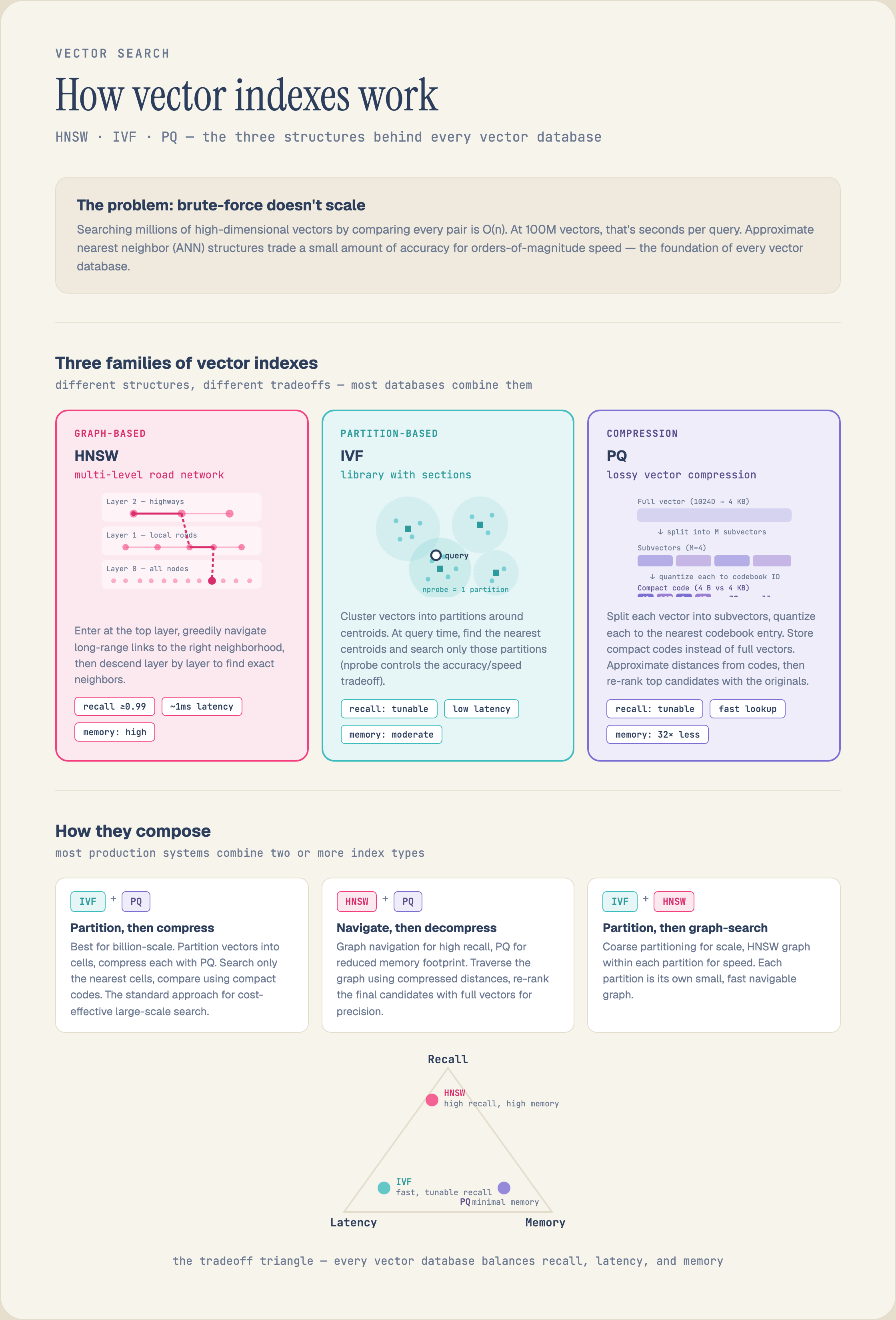
Partition the vector space into \(C\) clusters (cells) using k-means. At query time, find the \(p\) nearest cluster centroids, then search only the vectors in those clusters.
import faiss

d = 768          # embedding dimension
n_cells = 4096   # number of Voronoi cells
n_probe = 32     # cells to search at query time

quantizer = faiss.IndexFlatL2(d)
index = faiss.IndexIVFFlat(quantizer, d, n_cells)
index.train(training_vectors)    # runs k-means
index.add(all_vectors)

index.nprobe = n_probe
distances, ids = index.search(query, k=10)
The Math
K-means partitions \(n\) vectors into \(C\) Voronoi cells. The average cell contains \(n/C\) vectors. If you probe \(p\) cells, you search \(p \cdot n/C\) vectors instead of \(n\).
For \(C = 4096\) and \(p = 32\), you search only \(32/4096 = 0.78\%\) of the dataset. The overhead is finding the nearest centroids: \(O(C \cdot d)\), which is fast when \(C \ll n\).
The accuracy-speed trade-off is controlled entirely by \(nprobe\):
| nprobe (% of C) | Recall@10 (typical) | Relative Latency |
| 1 (0.02%) | 45-60% | 1x |
| 8 (0.2%) | 80-90% | 8x |
| 32 (0.8%) | 95-98% | 32x |
| 128 (3.1%) | 99%+ | 128x |
IVF + Product Quantization (IVF-PQ)
The brute-force scan within each cell is still \(O(
| cell |
PQ splits the vector into \(m\) sub-vectors of \(d/m\) dimensions each. Each sub-vector is quantized to one of 256 centroids (1 byte). The total code length is \(m\) bytes. Distance computation uses precomputed lookup tables, reducing cost from \(O(d)\) to \(O(m)\) per vector.
m = 48   # sub-quantizers (must divide d)
index = faiss.IndexIVFPQ(quantizer, d, n_cells, m, 8)  # 8 bits per sub-quantizer
index.train(training_vectors)
index.add(all_vectors)
When to Use IVF
IVF excels when:
The main weakness: k-means cluster boundaries are rigid. Vectors near the boundary of two cells may be missed if you do not probe both. This is why \(nprobe > 1\) is always necessary for good recall.
Algorithm 3: HNSW (Hierarchical Navigable Small World)
Core Idea
HNSW is a multi-layer graph where each vector is a node. Similar vectors are connected by edges. Search starts at the top layer (sparse, long-range connections) and descends to the bottom layer (dense, local connections), greedy-walking toward the query at each level.
The name comes from the "small world" property of the graph: most node pairs can be reached in a small number of hops, even in very large graphs.
Construction
When inserting a vector \(v\):
1. Assign a random level \(l\) drawn from a geometric distribution: \(l = \lfloor -\ln(uniform(0,1)) \cdot m_L \rfloor\), where \(m_L = 1/\ln(M)\). Most vectors live only on layer 0; a few reach higher layers.
2. Find neighbors on each layer. Starting from the entry point at the top layer, greedily descend to layer \(l\), then on each layer from \(l\) down to 0, find the \(M\) closest vectors and create bidirectional edges.
3. Prune connections. Each node keeps at most \(M\) neighbors per layer (\(2M\) on layer 0). A heuristic selects diverse neighbors — not just the closest, but neighbors that cover different directions in the space.
Search
function search(query, k, ef):
    candidates = entry_point
    for layer in [top_layer .. 1]:
        candidates = greedy_walk(query, candidates, 1, layer)
    candidates = greedy_walk(query, candidates, ef, layer=0)
    return top-k from candidates
The \(ef\) parameter (expansion factor) controls the accuracy-speed trade-off. A larger \(ef\) explores more nodes, increasing recall at the cost of latency:
Three properties make HNSW the default choice for sub-10-million-vector workloads:
1. No training step. Unlike IVF, there is no k-means clustering. Vectors can be inserted one at a time, making HNSW natural for real-time indexing.
2. Logarithmic scaling. The expected number of distance computations per query is \(O(\log n)\) hops across layers, with \(O(ef \cdot \log n)\) total comparisons. This holds up well to ~100M vectors.
3. High recall at low latency. HNSW consistently achieves 95%+ recall@10 in under 1ms on million-scale datasets. No other in-memory algorithm matches this combination.
Memory: Each vector needs ~\(M \cdot 8\) bytes of overhead for the graph structure (neighbor lists). With \(M = 32\), that is 256 bytes per vector on top of the vector itself. For a billion 768-dim vectors, the graph alone is 256 GB.
Build time: Inserting \(n\) vectors is \(O(n \cdot M \cdot \log n)\), which can take hours at billion scale.
No native disk support: HNSW assumes all vectors and the graph fit in RAM. Memory-mapped approaches work but degrade latency significantly.
| ef | Recall@10 | QPS (1M vectors, 768d) |
| 16 | ~85% | ~8,000 |
| 64 | ~95% | ~3,000 |
| 256 | ~99% | ~800 |
| 512 | ~99.5% | ~400 |
Why HNSW Dominates In-Memory Search
Three properties make HNSW the default choice for sub-10-million-vector workloads:
1. No training step. Unlike IVF, there is no k-means clustering. Vectors can be inserted one at a time, making HNSW natural for real-time indexing.
2. Logarithmic scaling. The expected number of distance computations per query is \(O(\log n)\) hops across layers, with \(O(ef \cdot \log n)\) total comparisons. This holds up well to ~100M vectors.
3. High recall at low latency. HNSW consistently achieves 95%+ recall@10 in under 1ms on million-scale datasets. No other in-memory algorithm matches this combination.
The Downsides
HNSW in Practice
import hnswlib

dim = 768
num_elements = 1_000_000
M = 32              # connections per node
ef_construction = 200   # construction-time expansion factor

index = hnswlib.Index(space='cosine', dim=dim)
index.init_index(max_elements=num_elements, M=M, ef_construction=ef_construction)
index.add_items(vectors, ids)

index.set_ef(64)    # query-time expansion factor
labels, distances = index.knn_query(query_vector, k=10)
Algorithm 4: Vamana / DiskANN
The Billion-Scale Problem
HNSW needs all data in RAM. At a billion vectors with 768 dimensions, that is ~3 TB for vectors plus 256 GB for the graph. Even with quantization, you are looking at $50,000+/month in cloud RAM costs.
Vamana (the algorithm behind Microsoft's DiskANN) solves this by building an HNSW-like graph but optimizing it for SSD access patterns. Vectors stay on disk; only a compressed navigation graph lives in RAM.
How It Works
1. Build a single-layer graph (unlike HNSW's multi-layer structure). The graph has degree \(R\) (typically 32-64) per node.
2. Optimize edge selection using a medoid-seeded greedy construction that produces shorter average path lengths than HNSW's random-level construction. The key innovation: Vamana explicitly optimizes for the "navigability" of the graph — every node should be reachable from the entry point in a small number of hops.
3. Store quantized vectors in RAM (for distance computation during navigation) and full-precision vectors on SSD (for final reranking). A typical setup: 32-byte PQ codes in RAM (32 GB for 1B vectors) + full vectors on NVMe SSD.
4. Beam search with SSD prefetching. Instead of HNSW's greedy walk, Vamana uses beam search with a width of \(W\). When the beam visits a node, it asynchronously prefetches that node's neighbors from SSD while computing distances for the current batch. This hides SSD latency behind computation.
Performance
| Scale | Recall@10 | Latency (p99) | RAM per Vector |
| 100M | 95% | ~1ms | ~32 bytes |
| 1B | 95% | ~3-5ms | ~32 bytes |
| 10B | 95% | ~8-12ms | ~32 bytes |
When to Use DiskANN
DiskANN is the right choice when:
The trade-off: build time is longer (hours to days for billion-scale), and the index is harder to update incrementally than HNSW.
Combining Algorithms: Production Architectures
Real systems rarely use a single algorithm. Here are three common patterns:
Pattern 1: HNSW + Scalar Quantization (Hot Tier)
For datasets under ~50M vectors where latency must be <1ms:
Full vectors (float32) → SQ8 quantized (int8, 4x smaller)
                       → HNSW graph (M=32, ef=64)
                       → Re-rank top-100 with full-precision vectors
Memory: ~1 KB per vector. At 10M vectors: ~10 GB RAM. All major vector databases default to this.
For 50M-1B vectors where latency can be 5-20ms:
Pattern 2: IVF-PQ + HNSW Coarse Quantizer (Warm Tier)
For 50M-1B vectors where latency can be 5-20ms:
Full vectors → PQ compressed (48 bytes each)
             → IVF with 65536 cells
             → HNSW index over the 65536 centroids (for fast cell selection)
             → Scan matching cells using PQ distance tables
             → Re-rank top-100 with full vectors (optional, from disk)
Memory: ~50 bytes per vector. At 500M vectors: ~25 GB RAM. This is what FAISS calls IndexIVFPQ with an HNSW quantizer.
For billion-scale with metadata filters:
Pattern 3: DiskANN + Filtered Search (Cold/Archive Tier)
For billion-scale with metadata filters:
Full vectors on SSD → PQ codes in RAM (32 bytes each)
                    → Vamana graph on SSD
                    → Label-constrained beam search
                    → Final re-rank from SSD
Memory: ~32 bytes per vector. At 5B vectors: ~160 GB RAM + ~20 TB SSD. DiskANN natively supports filtered search by incorporating filter predicates into the beam search — only expanding nodes that match the filter.
Under 10M vectors: HNSW with scalar quantization. No contest.
10M-100M vectors: HNSW if you can afford the RAM; IVF-PQ if you cannot.
100M-10B vectors: DiskANN/Vamana for low-latency; IVF-PQ for batch/offline workloads.
Streaming/real-time insert: HNSW (no rebuild needed) or LSH (constant-time insert).
When an AI agent searches a multimodal index — querying images by text, finding video moments by description, or matching audio clips — the underlying ANN algorithm determines three things the agent cares about:
1. Latency budget: An agent making 50 retrieval calls per reasoning chain needs sub-10ms search. HNSW or DiskANN.
2. Recall reliability: If the agent misses a relevant document, its reasoning may be wrong. Target 95%+ recall by tuning \(ef\) (HNSW), \(nprobe\) (IVF), or beam width (DiskANN).
3. Mixed-modality filtering: "Find images of red cars from the last 24 hours" combines vector similarity with metadata filters. DiskANN handles this natively; HNSW and IVF require post-filtering (search more, then filter) or pre-filtering (filter first, then search the subset).
Choosing the Right Algorithm
| Factor | LSH | IVF-PQ | HNSW | DiskANN |
| Recall@10 at 1ms | 70-80% | 85-92% | 95-99% | N/A (>1ms) |
| Recall@10 at 5ms | 85-90% | 95-98% | 99%+ | 95% |
| Memory per vector | ~100B | ~50B | ~3KB | ~32B |
| Max practical scale (RAM) | Unlimited | 5B+ | 50M | 10B+ |
| Insert latency | \(O(1)\) | Requires re-train | \(O(M \cdot \log n)\) | Batch rebuild |
| Filter support | Hash on metadata | Post-filter | Post-filter | Native |
| Build time (1B vectors) | Minutes | Hours | Hours | Hours-Days |
10M-100M vectors: HNSW if you can afford the RAM; IVF-PQ if you cannot.
100M-10B vectors: DiskANN/Vamana for low-latency; IVF-PQ for batch/offline workloads.
Streaming/real-time insert: HNSW (no rebuild needed) or LSH (constant-time insert).
How This Applies to Multimodal Agent Search
When an AI agent searches a multimodal index — querying images by text, finding video moments by description, or matching audio clips — the underlying ANN algorithm determines three things the agent cares about:
1. Latency budget: An agent making 50 retrieval calls per reasoning chain needs sub-10ms search. HNSW or DiskANN.
2. Recall reliability: If the agent misses a relevant document, its reasoning may be wrong. Target 95%+ recall by tuning \(ef\) (HNSW), \(nprobe\) (IVF), or beam width (DiskANN).
3. Mixed-modality filtering: "Find images of red cars from the last 24 hours" combines vector similarity with metadata filters. DiskANN handles this natively; HNSW and IVF require post-filtering (search more, then filter) or pre-filtering (filter first, then search the subset).
Example: Agent Perception Pipeline with Mixpeek
from mixpeek import Mixpeek

client = Mixpeek(api_key="YOUR_KEY")

# The ANN algorithm is abstracted away —
# Mixpeek selects HNSW, IVF-PQ, or DiskANN
# based on your namespace size and query pattern.

# Text → multimodal search (searches image, video, and text embeddings)
results = client.search(
    namespace="product-catalog",
    queries=[
        {
            "type": "text",
            "value": "red sports car on a mountain road",
            "field_name": "embedding"
        }
    ],
    filters={
        "AND": [
            {"field": "created_at", "operator": "gte", "value": "2026-05-01"},
            {"field": "modality", "operator": "eq", "value": "image"}
        ]
    },
    limit=20
)

# The response includes similarity scores from the ANN search
for result in results:
    print(f"{result['score']:.4f}  {result['file_name']}")
Under the hood, the search API routes to the appropriate index tier based on namespace size and query characteristics. Small namespaces use HNSW for minimum latency; large namespaces use IVF-PQ or DiskANN for memory efficiency. The accuracy-speed knobs (\(ef\), \(nprobe\), beam width) are auto-tuned based on the recall target in your namespace configuration.
The ANN Benchmarks project provides standardized comparisons across algorithms and implementations. Key metrics to track:
Recall@10 vs. QPS: the fundamental trade-off curve. Plot it for your data.
Index build time: matters for how fast you can re-index after embedding model updates.
Memory footprint: the cost driver at scale.
Tail latency (p99): more important than average latency for agent reliability. HNSW has tighter p99 than IVF because IVF cell sizes vary.
When evaluating, always benchmark on YOUR data. ANN algorithm performance depends heavily on the intrinsic dimensionality and clustering structure of the vector space. Embeddings from different models produce very different search characteristics.
Embedding Quantization & Compression -- the compression techniques (Matryoshka, BQ, PQ) that pair with these index structures
Multi-Stage Retrieval -- how agents chain coarse and fine retrieval
Late Interaction Retrieval -- ColBERT-style multi-vector search and its indexing implications
Hybrid Search -- combining keyword and vector search
Benchmarking Your Own Index
The ANN Benchmarks project provides standardized comparisons across algorithms and implementations. Key metrics to track:
When evaluating, always benchmark on YOUR data. ANN algorithm performance depends heavily on the intrinsic dimensionality and clustering structure of the vector space. Embeddings from different models produce very different search characteristics.